Distributed Decentralized Control for Satellite Mega-Constellations
Updated:
Application of a novel distributed decentralized Receding Horizon Control (RHC) framework to onboard orbit control of very large-scale constellations of satellites, illustrated in particular for a shell of the Starlink mega-constellation.
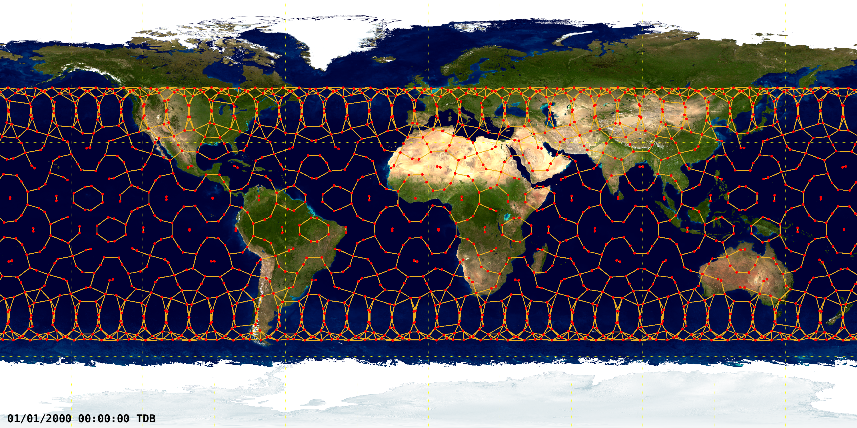
A novel distributed decentralized Receding Horizon Control (RHC) for very large-scale networks was proposed in [1]. In this example, which is also described thoroughly in [1], this solution is applied to the satellite mega-constellation onboard orbit control problem. An illustrative mega-constellation of a single shell inspired in the first shell of the Starlink constellation to be deployed is considered. The constellation is a Walker \(53.0º:1584/72/17\). A snapshot of ground track and inter-satellite links (ISL) of the simulated constellation at 0 TDB seconds since J2000 is depicted below.
High fidelity simulation
The realistic nonlinear numeric simulation is computed making use of the high fidelity open-source TU Delft’s Astrodynamic Toolbox (TUDAT). The documentation is available at https://docs.tudat.space/ and source code at https://github.com/tudat-team/tudat-bundle/. The orbit propagation of the satellites of the constellation accounts for several perturbations. The parameters that fully characterize the constellation, as well as the perturbations considered in the simulation, are detailed in [1].
The control feedback computation is carried out in MATLAB. The simulation environment relies on an interface between a C++ TUDAT application and MATLAB to define a thrust feedback control law. The architecture of the overall environment is shown below.

This interface is powered by the tudat-matlab-thrust-feedback package available at github.com/decenter2021/tudat-matlab-thrust-feedback.
The TUDAT application source-code can be found at Examples/DistributedDecentralizedRHCStarlink. For more details on how to setup and run the simulation and on the intricacies of the thruster actuation feedback, see the documentation of tudat-matlab-thrust-feedback.
Implementation of distributed decentralized RHC
The main steps of the simulation are described below. Jump to Results to see the implementation results.
To open this example execute the following command in the MATLAB command window
open DDRHCStarlink
The script that implements the control law in the simulation environment is Examples/DistributedDecentralizedRHCStarlink/DDELQR_iteration_routine.
First, convert the cartesian coordinates to mean relative orbital elements
%% Input:   t
%           x_t dim: 7N x 1
% Output:   MPC_u dim: 3 x N

%% Check redefinition of anchor
% Compute mean orbital elements
OE_t = zeros(n_single,N);
%for i = 1:N
parfor i = 1:N
    % With package osculating2mean
    aux = rv2OEOsc(x_t((i-1)*(n_single+1)+1:i*(n_single+1)-1));
    OE_t(:,i) = OEOsc2OEMeanEUK(t,aux,degree_osculating2mean);
end
% Condition for nominal anchor redefinition
% Define nominal anchor just by the initial state
if t < Tctrl/2 % Did not use t < 0 to avoid numerical issues
    fprintf('@MATLAB controller: Redefining nominal anchor at t = %g s.\n',t);
    [u0,Omega0] = nominalConstellationAnchor(OE_t([2 6],:),walkerParameters);
    t0 = t;
    walkerAnchor = [t0; u0; Omega0];
end

%% Transformation to relative obit elements
dalpha_t = zeros(n_single,N);
parfor i = 1:N
%for i = 1:N
    dalpha_t(:,i) = OEMean2OERel(OE_t(:,i),...
         nominalConstellationOEMean(t,i,walkerParameters,semiMajorAxis,walkerAnchor,0));
end
Then, compute a new RHC window if required
%% Check if a new MPC window needs to be computed
% Keep using the current window
if MPC_currentWindowGain < MPC_d && t > Tctrl/2
MPC_currentWindowGain = MPC_currentWindowGain+1;
% Compute a new window and use the first gain
else
MPC_currentWindowGain = 1;
%% Compute new MPC window
fprintf('@MATLAB controller: Computing new MPC window starting at t = %g s.\n',t);
%% MPC centralized backwards loop
% Initializations of dynamics matrices and topology for t = MPC_T
tau = MPC_T;
% Time instant (s) of MPC iteration
t_tau = t+tau*Tctrl;
% Predict nominal contellation at MPC iteration
OEMeanNominal_tau = nominalConstellationOEMean(t_tau,1:N,walkerParameters,semiMajorAxis,walkerAnchor,0);
% Scheduled time of communication regarding this instant
t_com = t - (tau+2)*Tt;
OEMeanNominal_t_com = nominalConstellationOEMean(t_com,1:N,walkerParameters,semiMajorAxis,walkerAnchor,0);
xNominal_tau = zeros(n_single,N);
xNominal_t_com = zeros(n_single,N);
parfor i = 1:N
xNominal_tau(:,i) = OEOsc2rv(OEMeanEU2OEOsc(OEMeanNominal_tau(:,i)));
xNominal_t_com(:,i) = OEOsc2rv(OEMeanEU2OEOsc(OEMeanNominal_t_com(:,i)));
end
% Predict topology
% With communication restrictions
% Compute in-neighbourhood
parfor i = 1:N
% If there were no restrictions
aux = LEOConstellationTrackingGraph_DMinus(i,xNominal_tau,trackingRange,trackingmaxInNeighbourhood);
% Communication restriction mask
mask = false(size(aux));
for l = 1:length(aux)
if norm(xNominal_t_com(1:3,i)-xNominal_t_com(1:3,aux(l))) < LOSRange
mask(l) = true;
end
end
% Apply mask
Di_tau_minus{i,1} = aux(mask);
end
% Without communication restrictions
% % Compute in-neighbourhood
% parfor i = 1:N
% Di_tau_minus{i,1} = LEOConstellationTrackingGraph_DMinus(i,xNominal_tau,trackingRange,trackingmaxInNeighbourhood);
% end
% Compute out-neighbourhood
parfor i = 1:N
Di_tau{i,1} = LEOConstellationTrackingGraph_DPlus(i,xNominal_tau,trackingRange,Di_tau_minus);
end
% Predict output dynamics and state weights
%for i = 1:N
parfor i = 1:N
% Predict output dynamics and state weights
[Haux,Q{i,1},~,o(i)] = LEOConstellationTrackingDynamics(i,Di_tau_minus,inclination);
aux = 1;
% Temporary variable to allow paralelization of cell H
H_tmp = cell(1,N);
for j = Di_tau_minus{i,1}'
H_tmp{1,j} = Haux{aux,1};
aux = aux + 1;
end
H(i,:) = H_tmp;
end
% MPC iterations start only at t = MPC_T-1
for tau = MPC_T-1:-1:0
%% Step 1. Predict topology and distributed dynamics
% Time instant (s) of MPC iteration
t_tau = t+tau*Tctrl;
%% 1.1 Predict nominal constellation
% Predict nominal contellation at MPC iteration
OEMeanNominal_tau = nominalConstellationOEMean(t_tau,1:N,walkerParameters,semiMajorAxis,walkerAnchor,0);
% Scheduled time of communication regarding this instant
t_com = t - (tau+2)*Tt;
OEMeanNominal_t_com = nominalConstellationOEMean(t_com,1:N,walkerParameters,semiMajorAxis,walkerAnchor,0);
xNominal_tau = zeros(n_single,N);
xNominal_t_com = zeros(n_single,N);
parfor i = 1:N
xNominal_tau(:,i) = OEOsc2rv(OEMeanEU2OEOsc(OEMeanNominal_tau(:,i)));
xNominal_t_com(:,i) = OEOsc2rv(OEMeanEU2OEOsc(OEMeanNominal_t_com(:,i)));
end
%% 1.2 Predict tracking topology for tau
% Store topology of last iteration (tau+1)
Di_tau_1 = Di_tau;
% With communication restrictions
% Compute in-neighbourhood
parfor i = 1:N
% If there were no restrictions
aux = LEOConstellationTrackingGraph_DMinus(i,xNominal_tau,trackingRange,trackingmaxInNeighbourhood);
% Communication restriction mask
mask = false(size(aux));
for l = 1:length(aux)
if norm(xNominal_t_com(1:3,i)-xNominal_t_com(1:3,aux(l))) < LOSRange
mask(l) = true;
end
end
% Apply mask
Di_tau_minus{i,1} = aux(mask);
end
% Without communication restrictions
% Compute in-neighbourhood
% parfor i = 1:N
% Di_tau_minus{i,1} = LEOConstellationTrackingGraph_DMinus(i,xNominal_tau,trackingRange,trackingmaxInNeighbourhood);
% end
% Compute out-neighbourhood
parfor i = 1:N
Di_tau{i,1} = LEOConstellationTrackingGraph_DPlus(i,xNominal_tau,trackingRange,Di_tau_minus);
end
%% Step 2: Recompute covarinaces (Compute P(tau+1) )
if decentralized
P_kl_prev = P_kl;
if tau ~= MPC_T-1
% Computations done distributedly across agents
%for i = 1:N
parfor i = 1:N
P_kl{i,1} = newCovarianceStorage(Di_tau{i,1});
% Compute each block of P
for j = 1:size(P_kl{i,1},1)
p = P_kl{i,1}{j,1}(1);
q = P_kl{i,1}{j,1}(2);
Cp = zeros(length(Di_tau{p,1})*n_single,n_single);
Cq = zeros(length(Di_tau{q,1})*n_single,n_single);
Prs = zeros(length(Di_tau{p,1})*n_single,length(Di_tau{q,1})*n_single);
lossPrs = 0;
count_r = 0;
% Sum over indices r ans s
% Build matrix P_rs, C_p, and Cq for each (p,q)
for r = Di_tau_1{p,1}'
if p == q
count_s = count_r;
for s = Di_tau_1{q,1}(count_r+1:end)'
% Get the P_rs computation available to i
[aux,loss] = searchP(i,r,s,P_kl_prev,Di_tau_1);
Prs(count_r*n_single+1:(count_r+1)*n_single,count_s*n_single+1:(count_s+1)*n_single)=...
aux;
if r ~= s
Prs(count_s*n_single+1:(count_s+1)*n_single,count_r*n_single+1:(count_r+1)*n_single)=...
Prs(count_r*n_single+1:(count_r+1)*n_single,count_s*n_single+1:(count_s+1)*n_single)';
end
lossPrs = lossPrs + loss;
count_s = count_s + 1;
end
else
count_s = 0;
for s = Di_tau_1{q,1}'
% Get the P_rs computation available to i
[aux,loss] = searchP(i,r,s,P_kl_prev,Di_tau_1);
Prs(count_r*n_single+1:(count_r+1)*n_single,count_s*n_single+1:(count_s+1)*n_single)=...
aux;
if count_r == 0
%Cq(count_s*n_single+1:(count_s+1)*n_single,:) = A{q,1}*(q==s)-B{s,1}*getK(MPC_K{s,tau+2},q);
Cq(count_s*n_single+1:(count_s+1)*n_single,:) = A{q,1}*(q==s)-B{s,1}*K_tau_1{q,1}{count_s+1,1};
end
lossPrs = lossPrs + loss;
count_s = count_s + 1;
end
end
Cp(count_r*n_single+1:(count_r+1)*n_single,:) = A{p,1}*(p==r)-B{r,1}*K_tau_1{p,1}{count_r+1,1};
count_r = count_r + 1;
end
% If p == q then, P_rs should be positive definite
if p == q
% If p == q then, P_rs should be positive definite
Prs = forcePositiveDefiniteness(Prs);
Cq = Cp;
end
% Intersection of D_p+ and D_q+
[r_cap_pq,r_cap_pq_idxp,r_cap_pq_idxq] = intersect(Di_tau_1{p,1},Di_tau_1{q,1});
aux = zeros(n_single,n_single);
for l = 1:length(r_cap_pq)
% parfor does not allow to assign a variable
% named 'r'
r_ = r_cap_pq(l);
r_idxp = r_cap_pq_idxp(l);
r_idxq = r_cap_pq_idxq(l);
aux = aux + H{r_,p}'*Q{r_,1}*H{r_,q} + K_tau_1{p,1}{r_idxp,1}'*R{r_,1}*K_tau_1{q,1}{r_idxq,1};
% + getK(MPC_K{r_,tau+2},p)'*R{r_,1}*getK(MPC_K{r_,tau+2},q);
end
P_kl{i,1}{j,2} = Cp'*Prs*Cq + aux;
% Update loss
P_kl{i,1}{j,3} = lossPrs;
end
end
else
% Computations done distributedly across agents
%for i = 1:N
parfor i = 1:N
P_kl{i,1} = newCovarianceStorage(Di_tau{i,1});
% Compute each block of P
for j = 1:size(P_kl{i,1},1)
p = P_kl{i,1}{j,1}(1);
q = P_kl{i,1}{j,1}(2);
% Intersection of D_p+ and D_q+
[r_cap_pq,~] = intersect(Di_tau_1{p,1},Di_tau_1{q,1});
aux = zeros(n_single,n_single);
for r = r_cap_pq'
aux= aux + H{r,p}'*Q{r,1}*H{r,q};
end
P_kl{i,1}{j,2} = aux;
% Update loss (not necessary, it is set to 0 on creation)
% P_kl{i,1}{j,3} = 0;
end
end
end
else
% Centralized version below:
% 2.1.1 Compute global matrices (H(tau+1), Q(tau+1), R(tau+1), K(tau+1), B(tau+1), A(tau+1))
% Init matrices
og = sum(o)*o_single_rel+N*o_single_self;
Hg = zeros(og,N*n_single);
Qg = zeros(og);
% Build matrices
aux = 0;
for i = 1:N
for j = Di_tau_1{i,1}'
Hg(aux+1:aux+o(i)*o_single_rel + o_single_self,(j-1)*n_single+1:(j-1)*n_single+n_single) = H{i,j};
end
Qg(aux+1:aux+o(i)*o_single_rel + o_single_self, aux+1:aux+o(i)*o_single_rel + o_single_self) = Q{i,1};
aux = aux+o(i)*o_single_rel + o_single_self;
end
% Compute P(tau+1)
if tau ~= MPC_T-1
P_tau_1 = Hg'*Qg*Hg + Kg'*Rg*Kg + (Ag-Bg*Kg)'*P_tau_1*(Ag-Bg*Kg);
else
P_tau_1 = Hg'*Qg*Hg;
end
end
%% Step 3: Predict dynamic and output dynamics matricexs for tau (A(tau), B(tau), R(tau))
%for i = 1:N
parfor i = 1:N
% Predict dynamics
[A{i,1},B{i,1}] = STMSatellite(OEMeanNominal_tau(:,i),Tctrl);
% Predict output dynamics, state weights, and input weights
[Haux,Q{i,1},R{i,1},o(i)] = LEOConstellationTrackingDynamics(i,Di_tau_minus,inclination);
aux = 1;
% Temporary variable to allow paralelization of cell H
H_tmp = cell(1,N);
for j = Di_tau_minus{i,1}'
H_tmp{1,j} = Haux{aux,1};
aux = aux + 1;
end
H(i,:) = H_tmp;
end
%% Step 4: Compute gains
if decentralized
% Decentralized gain computation
%for i = 1:N
parfor i = 1:N
% Compute augmented innovation covariance matrix
Si = zeros(m_single*length(Di_tau{i,1}));
% Compute augmented P_i tilde
Pi = zeros(m_single*length(Di_tau{i,1}),n_single);
count = 1;
for pidx = 1:length(Di_tau{i,1})
for qidx = pidx:length(Di_tau{i,1})
p = Di_tau{i,1}(pidx);
q = Di_tau{i,1}(qidx);
% Fill Si
Si((pidx-1)*m_single+1:(pidx-1)*m_single+m_single,(qidx-1)*m_single+1:(qidx-1)*m_single+m_single) = ...
B{p,1}'*P_kl{i,1}{count,2}*B{q,1} + (p==q)*R{p,1};
if pidx ~= qidx
Si((qidx-1)*m_single+1:(qidx-1)*m_single+m_single,(pidx-1)*m_single+1:(pidx-1)*m_single+m_single) = ...
Si((pidx-1)*m_single+1:(pidx-1)*m_single+m_single,(qidx-1)*m_single+1:(qidx-1)*m_single+m_single)';
end
% Fill Pi
if p == i || q == i
if p == i
Pi((qidx-1)*m_single+1:(qidx-1)*m_single+m_single,:) = B{q,1}'*P_kl{i,1}{count,2}'*A{i,1};
else
Pi((pidx-1)*m_single+1:(pidx-1)*m_single+m_single,:) = B{p,1}'*P_kl{i,1}{count,2}*A{i,1};
end
end
count = count + 1;
end
end
% Compute gains
Ki = Si\Pi;
% Fill K_tau_1
K_tau_1{i,1} = cell(length(Di_tau{i,1}),1);
for pidx = 1:length(Di_tau{i,1})
K_tau_1{i,1}{pidx,1} = Ki((pidx-1)*m_single+1:(pidx-1)*m_single+m_single,:);
end
end
else
% Centralized computation below
% 4.1 Compute global matrices (B, R, A)
Bg = zeros(n_single*N,m_single*N);
Rg = zeros(m_single*N);
Ag = zeros(n_single*N);
% Predict dynamics
for i = 1:N
Ag((i-1)*n_single+1:i*n_single,(i-1)*n_single+1:i*n_single) = A{i,1};
Bg((i-1)*n_single+1:i*n_single,(i-1)*m_single+1:i*m_single) = B{i,1};
Rg((i-1)*m_single+1:i*m_single,(i-1)*m_single+1:i*m_single) = R{i,1};
end
% 4.2 Compute gains
Sg = Bg'*P_tau_1*Bg + Rg;
Kg = Sg\Bg'*P_tau_1*Ag;
end
%% Step 3.5 Transmit gains
if decentralized
% Fill decentralized MPC gains k(tau)
if tau <= MPC_d
% If the topology is undirected the implementation below is
% more efficient
% for i = 1:N
% %parfor i = 1:N
% MPC_K{i,tau+1} = cell(length(Di_tau{i,1}),2); % MPC_K{i,tau+1} = cell(length(Di_tau_minus{i,1}),2);
% % They gains must be recived by agents in D_i-, but given
% % that, in this case in particular, the edges are
% % undirected, then we can use D_i+ (Di_tau) to index the
% % agents and retrieve the gains (it is more efficient)
% % Warning: if the topology is directed the code above must
% % be adapted (we have to compute and use Di_tau_minus)
% for pidx = 1:length(Di_tau{i,1}) % pidx = 1:length(Di_tau_minus{i,1})
% p = Di_tau{i,1}(pidx); % p = Di_tau_minus{i,1}(pidx);
% MPC_K{i,tau+1}{pidx,1} = p;
% i_idx = find(Di_tau{p,1}==i);
% MPC_K{i,tau+1}{pidx,2} = K_tau_1{p,1}{i_idx,1};
% end
% end
% If the topology is directed, then the implementation
% above is not valid
for i = 1:N
%parfor i = 1:N
MPC_K{i,tau+1} = cell(length(Di_tau_minus{i,1}),2);
for pidx = 1:length(Di_tau_minus{i,1})
p = Di_tau_minus{i,1}(pidx);
MPC_K{i,tau+1}{pidx,1} = p;
i_idx = find(Di_tau{p,1}==i);
MPC_K{i,tau+1}{pidx,2} = K_tau_1{p,1}{i_idx,1};
end
end
end
else
% Centralized below
% % For debug: fill K_tau_1 gains for the computation of P_tau_1 in the next MPC
% % iteration
% for i = 1:N
% K_tau_1{i,1} = cell(length(Di_tau{i,1}),1);
% for j = 1:length(Di_tau{i,1})
% p = Di_tau{i,1}(j);
% K_tau_1{i,1}{j,1} = Kg((p-1)*m_single+1:(p-1)*m_single+m_single,(i-1)*n_single+1:(i-1)*n_single+n_single);
% end
% end
%
% % For debug: enforce saprsity of global gain
% for i = 1:N
% for j = 1:N
% if sum(i==Di_tau{j,1}) == 0
% Kg((i-1)*m_single+1:(i-1)*m_single+m_single,(j-1)*n_single+1:(j-1)*n_single+n_single) = zeros(m_single,n_single);
% end
% end
% end
% Fill centralized MPC gains k(tau)
if tau <= MPC_d
for i = 1:N
MPC_K{i,tau+1} = cell(N,2);
for j = 1:N
MPC_K{i,tau+1}{j,1} = j;
MPC_K{i,tau+1}{j,2} = Kg((i-1)*m_single+1:i*m_single,(j-1)*n_single+1:j*n_single);
end
end
end
end
end
fprintf('@MATLAB controller: Computed new MPC window starting at t = %g s.\n',t);
end
Finally, compute the thrust of each satellite
%% Compute actuation
% Each satellite computes its actuation based on the known gains
%for i = 1:N
parfor i = 1:N
    % Auxiliary varibale to allow parallelization
    uaux = zeros(m_single,1);
    for j = 1:size(MPC_K{i,MPC_currentWindowGain},1)
        uaux = uaux - MPC_K{i,MPC_currentWindowGain}{j,2}*...
            dalpha_t(:,MPC_K{i,MPC_currentWindowGain}{j,1});
    end
    % Compute actuation force from actuation mass
    uaux = uaux*x_t(i*(n_single+1));
    % Saturate thrust
    uaux(uaux>Ct1) = Ct1;
    uaux(uaux<-Ct1) = -Ct1;
    % Assign thrust
    MPC_u(:,i) = uaux;
end
The auxiliary functions that are employed in the script above are included in the examples files, made available in the DECENTER toolbox. This script also makes use of the osculating2mean toolbox, which is included as well.
Results
The evolution of the global mean absolute error (MAE) for semi-major axis, eccentricity, inclination, mean argument of latitude, and longitude of ascending node is shown below.


The evolution of the mean absolute error (MAE), for satellite 1, in semi-major axis, inclination, and eccentricity is shown below.


The evolution of the 3-axis thrust input and trajectory of the error in mean argument of latitude and longitude of ascending node are shown below.


For a thorough analysis of these results, see [1].