Distributed Decentralized EKF for Satellite Mega-Constellations
Updated:
Application of a novel distributed decentralized EKF framework to the navigation of very large-scale constellations of satellites, illustrated in particular for a shell of the Starlink mega-constellation.
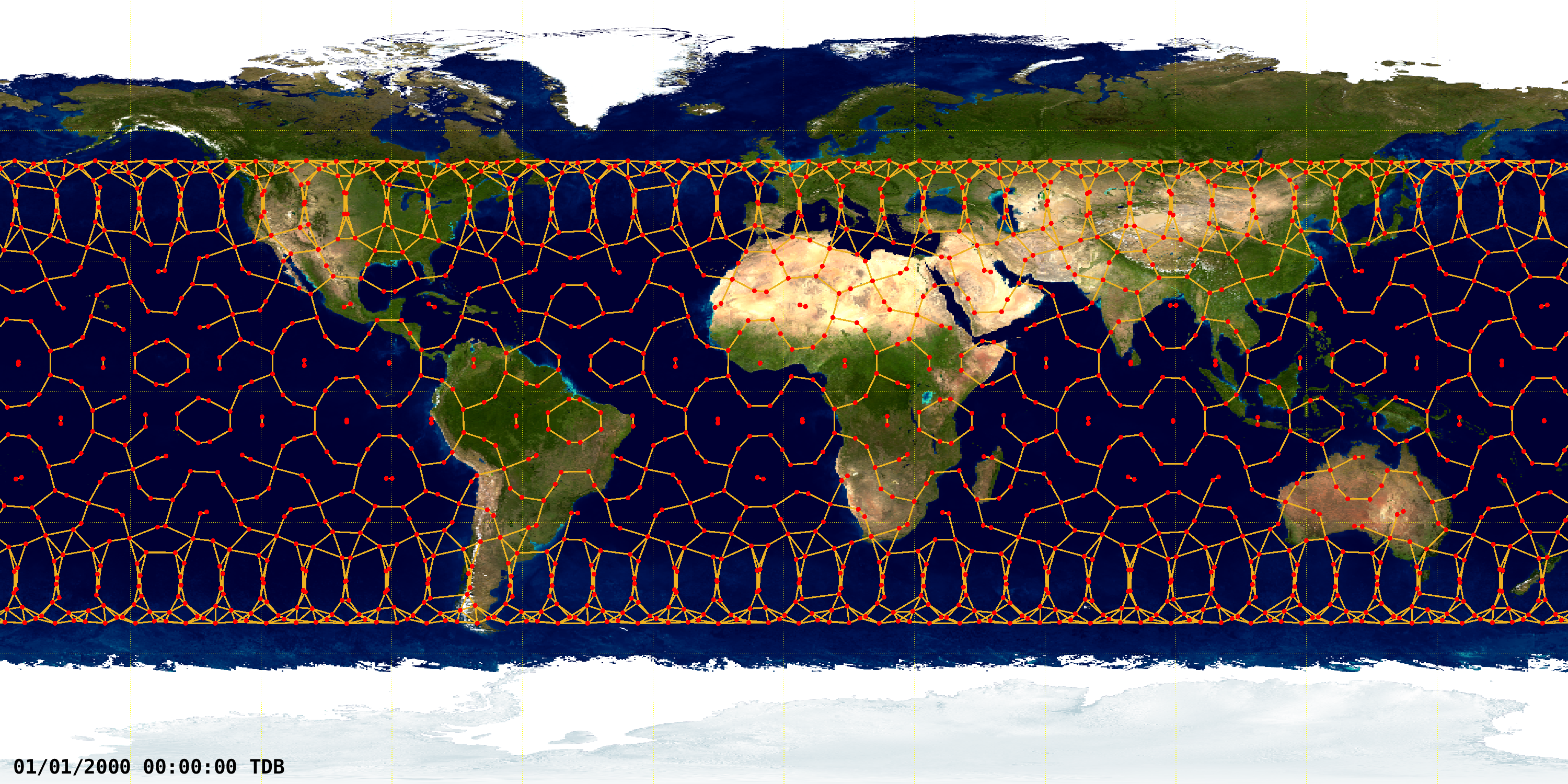
A novel distributed decentralized EKF framework for very large-scale networks was proposed in [1]. In this example, this solution is applied to the satellite mega-constellation navigation problem. An illustrative mega-constellation of a single shell inspired in the first shell of the Starlink constellation to be deployed is considered. The constellation is a Walker \(53.0º:1584/72/17\). A snapshot of ground track and inter-satellite links (ISL) of the simulated constellation at 0 TDB seconds since J2000 is depicted below.
This example is organized into two parts: i) simulation of the constellations making use of an high-fidelity propagator; and ii) implementation of the EKF to obtain a distributed navigation solution in a decentralized framework.
High fidelity simulation
The realistic nonlinear numeric simulation is computed making use of the high fidelity open-source TU Delft’s Astrodynamic Toolbox (TUDAT). The documentation is available at https://docs.tudat.space/ and source code at https://github.com/tudat-team/tudat-bundle/. The orbit propagation of the satellites of the constellation accounts for several perturbations. The parameters that fully characterize the constellation, as well as the perturbations considered in the simulation, are detailed in [1].
The TUDAT application source-code can be found at
Examples/DistributedDecentralizedEKFStarlinkConstellation/tudatSimulation.
The .mat output of a simulation of roughly 1 full orbital period can be downloaded (419 MB) here.
The TUDAT application source-code consists of a C++ script that simulates the orbital dynamics of a constellation of satellites. It also establishes a UDP connection with a server running on a MATLAB instance to obtain thruster actuation feedback. For more details on how to setup the simulation and on the intricacies of the thruster actuation feedback, see the dedicated GitHub repository.
Implementation of distributed decentralized EKF
The main steps of the simulation are described below. Jump to Results to see the implementation results.
To open this example execute the following command in the MATLAB command window
open DDEKFConstellationCart
First, initialize variables and import simulation data
%% Define constellation
numberOfPlanes = 72;
numberOfSatellitesPerPlane = 22;
% Maximum communication distance normalized by the arc length between
% staellites on the same orbit
ISLRange = 750e3;
minInNeighbourhood = 1;
maxInNeighbourhood = 3;
semiMajorAxis = 6921000;

% Number of satellites
N = numberOfPlanes*numberOfSatellitesPerPlane;

% Init dimensions of the dynamics of each satellite
o_single = 3;
n_single = 6;
fprintf("Constellation defined.\n");

%% Simulation
Ts = 1; % Sampling time (s)
Tsim = 5730;
ItSim = Tsim/Ts+1; % One week
% Load true data
load('./data/output_orb_2023_01_15.mat','x');

% Reduce dimension of imported data arrays
parfor i = 1:N
    x{i,1} = x{i,1}(:,1:ItSim);
end
fprintf("Constellation simulation uploaded.\n");

%% Filter simulation - variable definition
%%%% DEK simulation variables
% Estimate vector time series
x_hat = cell(N,1);
for i = 1:N
    x_hat{i,1} = zeros(n_single,ItSim);
end
x_hat_pred = cell(N,1);
% Output vector
y = cell(N,1);
% In neighbourhood
Fim = cell(N,1);
FimNew = cell(N,1);
FimHist = cell(ItSim-1,1);
% Access to inertial measurements (skip = 1)
Fii = [];
% count = 0;
% for i = 0:numberOfPlanes-1
%     j = i*numberOfSatellitesPerPlane+1+count;
%     count = count + 1;
%     count = rem(count,numberOfSatellitesPerPlane);
%     Fii = [Fii j];
% end
Fii = (1:N)';

% Data structures of the dynamics to emulate communication
A = cell(N,1);
Q = cell(N,1);
C = cell(N,N);
o = zeros(N,1);
R = cell(N,N);
% Covariance between nodes in F_i^-
P_kl = cell(N,1);
P_kl_pred = cell(N,1);
% Matrices S_ii
S = cell(N,1);
% Gains K_i
K = cell(N,1);

%% Filter simulation - covariance initializaton
%%%% Covariance initialization
% Initial estimation error covariance
P0_single = blkdiag(10^2*eye(3),0.1^2*eye(3));
%%%% Estimate initialization
for i = 1:N
    x_hat{i,1}(:,1) = x{i,1}(1:n_single,1)+ mvnrnd(zeros(n_single,1),P0_single)';
end

%% Evolution of feedback variables
trace_log = zeros(N,ItSim-1);
P_pos_log = zeros(N,ItSim-1,3);
Second, compute the estimate for each discrete-time instant
%% Filter simulation - filter iterations
fprintf("Simulating DEKF.\n");
fprintf("Iteration: %08d/%08d",1,ItSim);

for t = 1:ItSim-1
    % Update counter
    fprintf("\b\b\b\b\b\b\b\b\b\b\b\b\b\b\b\b\b%08d/%08d",t,ItSim-1);
    % To distribute less memory across cores define temporary variables
    parfor i = 1:N
        x_t1(:,i) = x{i,1}(1:n_single,t+1);
    end
    %% DEKF - Steps for each time-step for each satellite
    FimHist{t,1} = Fim;
    %% Step 1 - Predict the estimate, topology and compute linearized dynamics
%     % Before UKF
%     parfor i = 1:N
%         % x_hat_i(t+1|t)
%         % A_ii(t)
%         % Q_ii(t)
%         [x_hat_pred{i,1},A{i,1},Q{i,1}] = predictionCart(x_hat{i,1}(:,t),zeros(3,1),Ts);
%     end
    parfor i = 1:N
        Q{i,1} = QCartUT(x_hat{i,1}(:,t),zeros(3,1),Ts);
    end

    %% Step 2 - Predict the topology
    % Here we are using the real distance between satellites
    % We could, instead use an estimate, and if the satellite does not
    % communicate then we disregard it in function
    % LEOConstellationMeasurementGraphSynch
    aux = zeros(n_single,N);
    parfor i = 1:N
        aux(:,i) = x_t1(:,i);
    end
    parfor i = 1:N
        % Before limited number of neighbors
        % FimNew{i,1} = LEOConstellationMeasurementGraph(i,aux,ISLRange);
        % After limited number of neighbors
        FimNew{i,1} = LEOConstellationMeasurementGraph_limited(i,aux,ISLRange);
    end

    %% Step 3,4 - Communication
    %% Step 5 - Topology synch
    % Before limited number of neighbors
    FimNew = LEOConstellationMeasurementGraphSynch(FimNew);
    % After limited number of neighbors
    %FimNew = LEOConstellationMeasurementGraphSynch_limited(FimNew,minInNeighbourhood,maxInNeighbourhood);

    %% Step 6 - Update filtered covariance
    % P(t|t)
    if t > 1
        parfor i = 1:N
            P_kl{i,1} = newCovarianceStorage(FimNew{i,1});
            for j = 1:size(P_kl{i,1},1)
                p = P_kl{i,1}{j,1}(1);
                q = P_kl{i,1}{j,1}(2);
                Cp = zeros(n_single,length(FimNew{p,1})*n_single);
                Cq = zeros(n_single,length(FimNew{q,1})*n_single);
                Prs = zeros(length(FimNew{p,1})*n_single,length(FimNew{q,1})*n_single);
                lossPrs = 0;
                count_r = 0;
                % Sum over indices r ans s
                % Build matrix P_rs, C_p, and Cq for each (p,q)
                for r = Fim{p,1}'
                    if p == q
                        count_s = count_r;
                        for s = Fim{q,1}(count_r+1:end)'
                            % Get the P_rs computation available to i
                            [aux,loss] = searchP(i,p,q,r,s,P_kl_pred,Fim);
                            Prs(count_r*n_single+1:(count_r+1)*n_single,count_s*n_single+1:(count_s+1)*n_single)=...
                                aux;
                            if r ~= s
                                Prs(count_s*n_single+1:(count_s+1)*n_single,count_r*n_single+1:(count_r+1)*n_single)=...
                                    Prs(count_r*n_single+1:(count_r+1)*n_single,count_s*n_single+1:(count_s+1)*n_single)';
                            end
                            lossPrs = lossPrs + loss;
                            count_s = count_s + 1;
                        end
                    else
                        count_s = 0;
                        for s = Fim{q,1}'
                            % Get the P_rs computation available to i
                            [aux,loss] = searchP(i,p,q,r,s,P_kl_pred,Fim);
                            Prs(count_r*n_single+1:(count_r+1)*n_single,count_s*n_single+1:(count_s+1)*n_single)=...
                                aux;
                            if count_r == 0
                                Cq(:,count_s*n_single+1:(count_s+1)*n_single) = eye(n_single)*(q==s)-K{q,1}*C{q,s};
                            end
                            lossPrs = lossPrs + loss;
                            count_s = count_s + 1;
                        end
                    end
                    Cp(:,count_r*n_single+1:(count_r+1)*n_single) = eye(n_single)*(p==r)-K{p,1}*C{p,r};
                    count_r = count_r + 1;
                end

                if p == q
                    % If p == q then, P_rs should be positive definite
                    Prs = forcePositiveDefiniteness(Prs,0);
                    P_kl{i,1}{j,2} = K{p,1}*R{p,p}*K{p,1}'+Cp*Prs*Cp';
                    P_kl{i,1}{j,2} = (1/2)*(P_kl{i,1}{j,2}+P_kl{i,1}{j,2}');
                elseif sum(q == Fim{p,1}) % if p and q have a relative mesurment between them
                    P_kl{i,1}{j,2} = K{p,1}*R{p,q}*K{q,1}' + Cp*Prs*Cq';
                else
                    P_kl{i,1}{j,2} = Cp*Prs*Cq';
                end
                % Update loss
                P_kl{i,1}{j,3} = lossPrs;
            end
        end

    else
        % Covariance initialization
        for i = 1:N
            P_kl{i,1} = newCovarianceStorage(FimNew{i,1});
            % Repeated combinations
            for j = 1:size(P_kl{i,1},1)
                p = P_kl{i,1}{j,1}(1);
                q = P_kl{i,1}{j,1}(2);
                if p == q
                    P_kl{i,1}{j,2} = P0_single;
                else
                    P_kl{i,1}{j,2} = zeros(n_single,n_single);
                end
            end
        end
    end

    %% Step 7 - Update C and R
    % C_ij(t+1)
    % R_ij(t+1)
    parfor i = 1:N
        %[Caux,R{i,1},o(i)] = LEOConstellationOutputDynamics(i,FimNew{i,1},sum(Fii==i));
        [Caux,Raux,o(i)] = LEOConstellationOutputDynamics(i,FimNew,Fii);
        aux = 1;
        % Temporary variable to allow paralelization of cell C
        C_tmp = cell(1,N);
        for j = FimNew{i,1}'
            C_tmp{1,j} = Caux{aux,1};
            aux = aux + 1;
        end
        C(i,:) = C_tmp;
        % Temporary variable to allow paralelization of cell R
        aux = 1;
        for j = FimNew{i,1}'
            C_tmp{1,j} = Raux{aux,1};
            aux = aux + 1;
        end
        R(i,:) = C_tmp;
    end

%     %% Step 8 - Predict covariance (before UKF)
%     % P_i(pq)(t+1|t)
%     % S_ii(t+1)
%     % Ki(t+1)
%     P_kl_pred = P_kl;
%     parfor i = 1:N
%         for j = 1:size(P_kl{i,1},1)
%             p = P_kl_pred{i,1}{j,1}(1);
%             q = P_kl_pred{i,1}{j,1}(2);
%             % Local covariance prediction
%             P_kl_pred{i,1}{j,2} = A{p,1}*P_kl{i,1}{j,2}*A{q,1}';
%             if p == q
%                 % if p == q P_i(pq)(t+1|t) must be positive definite
%                 P_kl_pred{i,1}{j,2} = P_kl_pred{i,1}{j,2} + Q{p,1};
%                 P_kl_pred{i,1}{j,2} = (1/2)*(P_kl_pred{i,1}{j,2}+P_kl_pred{i,1}{j,2}');
%             end
%         end
%
%         % Compute innovation covarinace
%         Pi = zeros(length(FimNew{i,1})*n_single);
%         Ci = zeros(o_single*o(i),length(FimNew{i,1})*n_single);
%         idxi = 0;
%         countk = 0;
%         for k = FimNew{i,1}'
%             if k == i
%                 idxi = countk;
%             end
%             Ci(:,countk*n_single+1:(countk+1)*n_single) = C{i,k};
%             countl = countk;
%             for l = FimNew{i,1}(countk+1:end)'
%                 Pi(countk*n_single+1:(countk+1)*n_single,countl*n_single+1:(countl+1)*n_single)=...
%                     getP(P_kl_pred{i,1},k,l);
%                 if l ~= k
%                     Pi(countl*n_single+1:(countl+1)*n_single,countk*n_single+1:(countk+1)*n_single)=...
%                         Pi(countk*n_single+1:(countk+1)*n_single,countl*n_single+1:(countl+1)*n_single)';
%                 end
%                 countl = countl + 1;
%             end
%             countk = countk + 1;
%         end
%         % Pi must be positive definite
%         Pi = forcePositiveDefiniteness(Pi,0);
%         % Local computation of innovation covariance matrix
%         S{i,1} = R{i,i}+Ci*Pi*Ci';
%         S{i,1} = (1/2)*(S{i,1}+S{i,1}');
%         aux = Pi(idxi*n_single+1:(idxi+1)*n_single,:)*Ci';
%
%         % Compute the gain locally
%         K{i,1} = aux/S{i,1};
%
%     end

    %% Step 8 - Predict covariance (UKF)
    % P_i(pq)(t+1|t)
    % S_ii(t+1)
    % Ki(t+1)
    P_kl_pred = P_kl;
    parfor i = 1:N
        % Define local concatenated covariance matrices and local concatenated estimates
        % Take avatage of the loop to compute the concatenation of C
        x_hat_i = zeros(length(FimNew{i,1})*n_single,1);
        Pi = zeros(length(FimNew{i,1})*n_single);
        Ci = zeros(o_single*o(i),length(FimNew{i,1})*n_single);
        idxi = 0;
        countk = 0;
        for k = FimNew{i,1}'
            if k == i
                idxi = countk;
            end
            x_hat_i(countk*n_single+1:(countk+1)*n_single,1) = x_hat{i,1}(:,t);
            Ci(:,countk*n_single+1:(countk+1)*n_single) = C{i,k};
            countl = countk;
            for l = FimNew{i,1}(countk+1:end)'
                Pi(countk*n_single+1:(countk+1)*n_single,countl*n_single+1:(countl+1)*n_single)=...
                    getP(P_kl{i,1},k,l);
                if l ~= k
                    Pi(countl*n_single+1:(countl+1)*n_single,countk*n_single+1:(countk+1)*n_single)=...
                        Pi(countk*n_single+1:(countk+1)*n_single,countl*n_single+1:(countl+1)*n_single)';
                end
                countl = countl + 1;
            end
            countk = countk + 1;
        end
        % Pi must be positive definite
        Pi = forcePositiveDefiniteness(Pi,0);
        % Compute sigma points and weights
        % Wan, E.A. and Van Der Merwe, R., 2000, October. The unscented Kalman
        % filter for nonlinear estimation. In Proceedings of the IEEE 2000 Adaptive
        % Systems for Signal Processing, Communications, and Control Symposium
        % (Cat. No. 00EX373) (pp. 153-158). Ieee.
        % Julier, S.J. and Uhlmann, J.K., 2004. Unscented filtering and
        % nonlinear estimation. Proceedings of the IEEE, 92(3), pp.401-422.
        % Unscented transformation parameters
        L = length(x_hat_i);
        UTpar_alpha = 1e-3;
        UTpar_k = 0;
        UTpar_beta = 2;
        % Sigma points
        UTpar_lambda = (UTpar_alpha^2)*(L+UTpar_k)-L;
        P_sqrt = chol((L+UTpar_lambda)*Pi)';
        Ksi = [x_hat_i x_hat_i+P_sqrt x_hat_i-P_sqrt];
        % Weights
        W_m = [UTpar_lambda/(L+UTpar_lambda); ones(2*L,1)*1/(2*(L+UTpar_lambda))];
        W_c = W_m;
        W_c(1) = W_m(1) + 1-UTpar_alpha^2+UTpar_beta;
        % Propagate sigma points
        for l = 1:2*L+1
            for s = 1:length(FimNew{i,1})
                Ksi((s-1)*n_single+1:s*n_single,l) = predictionCartUT(Ksi((s-1)*n_single+1:s*n_single,l),zeros(3,1),Ts);
            end
        end
        % Compute mean
        x_hat_i = zeros(L,1);
        for l = 1:2*L+1
            x_hat_i = x_hat_i + W_m(l)*Ksi(:,l);
        end
        % Compute covariance
        Ksi = Ksi - x_hat_i;
        Pi = zeros(L,L);
        for l = 1:2*L+1
            Pi = Pi + W_c(l)*(Ksi(:,l)*Ksi(:,l)');
        end
        % Fill predicted estimate of the satellite
        x_hat_pred{i,1} = x_hat_i(idxi*n_single+1:(idxi+1)*n_single,1);
        % Add additive process noise and fill data structure with covariances
        countk = 0;
        for k = FimNew{i,1}'
            Pi(countk*n_single+1:(countk+1)*n_single,countk*n_single+1:(countk+1)*n_single) = ...
                Pi(countk*n_single+1:(countk+1)*n_single,countk*n_single+1:(countk+1)*n_single) + Q{k,1};
            countl = countk;
            for l = FimNew{i,1}(countk+1:end)'
                % Find the position on the data structure
                for s = 1:size(P_kl_pred{i,1})
                    if(sum(P_kl_pred{i,1}{s,1} == [k;l]) == 2)
                        P_kl_pred{i,1}{s,2} = ...
                            Pi(countk*n_single+1:(countk+1)*n_single,countl*n_single+1:(countl+1)*n_single);
                        break;
                    end
                end
                countl = countl + 1;
            end
            countk = countk + 1;
        end
        % Local computation of innovation covariance matrix
        S{i,1} = R{i,i}+Ci*Pi*Ci';
        S{i,1} = (1/2)*(S{i,1}+S{i,1}');
        aux = Pi(idxi*n_single+1:(idxi+1)*n_single,:)*Ci';
        % Compute the gain locally
        K{i,1} = aux/S{i,1};
    end

    %% Step 7 - Take the measurement
    % Correlated measurement noise generated locally
    for i = 1:N
        % Add error to each measurement relative to satellites in Fim of i
        y{i,1} = zeros(o(i)*o_single,1);
        % Counter for the number of the local output
        aux = 1;
        for j = 1:size(FimNew{i,1},1)
            % temporary variable to allow paralelization
            y_tmp = zeros(o(i)*o_single,1);
            % Number of satellite
            satj = FimNew{i,1}(j);
            if satj == i
                continue;
            end
            if satj > i
                y{i,1}((aux-1)*o_single+1:aux*o_single,1) = mvnrnd(zeros(o_single,1),R{i,i}((aux-1)*o_single+1:aux*o_single,(aux-1)*o_single+1:aux*o_single))';
            else
                % Find the number of the local output in j
                auxj = 1;
                for l = 1:size(FimNew{satj,1},1)
                    if FimNew{satj,1}(l) == i
                        break;
                    elseif FimNew{satj,1}(l) ~= satj
                        auxj = auxj + 1;
                    end
                end
                y{i,1}((aux-1)*o_single+1:aux*o_single,1) = -y{satj,1}((auxj-1)*o_single+1:auxj*o_single);
            end
            aux = aux + 1;
        end
        % Add inertial error
        if o(i)==aux % if has inertial measurment
            y{i,1}((aux-1)*o_single+1:aux*o_single,1) = mvnrnd(zeros(o_single,1),R{i,i}((aux-1)*o_single+1:aux*o_single,(aux-1)*o_single+1:aux*o_single))';
        end
    end
    % Take measurments
    parfor i = 1:N
        for j = FimNew{i,1}'
            y{i,1} = y{i,1} + C{i,j}*x_t1(:,j);
        end
    end

    %% Step 8 - Update the estimate
    parfor i = 1:N
        % Compute predicted output (it is linear in cartesian coodinates)
        y_hat = zeros(size(C{i,i},1),1);
        for j = FimNew{i,1}'
            y_hat = y_hat + C{i,j}*x_hat_pred{j,1};
        end
        % Update step
        x_hat{i,1}(:,t+1) = x_hat_pred{i,1}+K{i,1}*(y{i,1}-y_hat);
        Fim{i,1} = FimNew{i,1};
    end

    %% Log estimated trace
    parfor i = 1:N
        aux = getP(P_kl{i,1},i,i);
        trace_log(i,t) = trace(aux);
        for m = 1:3
            P_pos_log(i,t,m) = aux(m,m);
        end
    end
end
The auxiliary functions that are employed in the script above are defined in the main simulation script, made available in the DECENTER toolbox.
Results
The evolution of the position estimation error with the use of relative measurements, making use of the novel algorithm proposed in [1], for satellite 1, is shown below.

It is possible to note that, near the poles, there are more relative measurement links. Thus, near the poles, the estimation performance increases. This effect is also visible in the evolution of the trace of the estimation error covariance matrix and number of satellites in ISL range, for satellite 1.
